How to use the VoxelFields class

What are VoxelFields?

From a high-level perspective, evoxels is organized around two core abstractions: VoxelFields and VoxelGrid. VoxelFields provides a uniform, NumPy-based container for any number of 3D fields on the same regular grid, maximizing interoperability with image I/O libraries (e.g. tifffile, h5py, napari, scikit-image) and visualization tools (PyVista, VTK). VoxelGrid couples these fields to either a PyTorch or JAX backend, offering pre-defined boundary conditions, finite difference stencils and FFT libraries.

It is meant to organize, plot and export multiple fields on the same underlying grid (i.e. same shape, origin, spacing and grid convention).

Getting started

Import the evoxels library together with numpy

import evoxels as evo
import numpy as np

Create a voxel fields object and explore some of its properties

Nx, Ny, Nz = [20, 10, 5]
vf = evo.VoxelFields((Nx, Ny, Nz), domain_size=(Nx, Ny, Nz))
print("VoxelFields object is now defined as")
print(f" - grid with {vf.Nx} x {vf.Ny} x {vf.Nz} points,")
print(f" - defined with {vf.convention} grid convention.")
print(f" - Physical domain size {vf.domain_size}")
print(f" - and the resulting grid spacing {vf.spacing}")
print(f" - First grid point (origin) is located at {vf.origin}")
print(f" - Float precision of data is set to {vf.precision}")

VoxelFields object is now defined as
 - grid with 20 x 10 x 5 points,
 - defined with cell_center grid convention.
 - Physical domain size (20, 10, 5)
 - and the resulting grid spacing (1.0, 1.0, 1.0)
 - First grid point (origin) is located at (0.5, 0.5, 0.5)
 - Float precision of data is set to float32

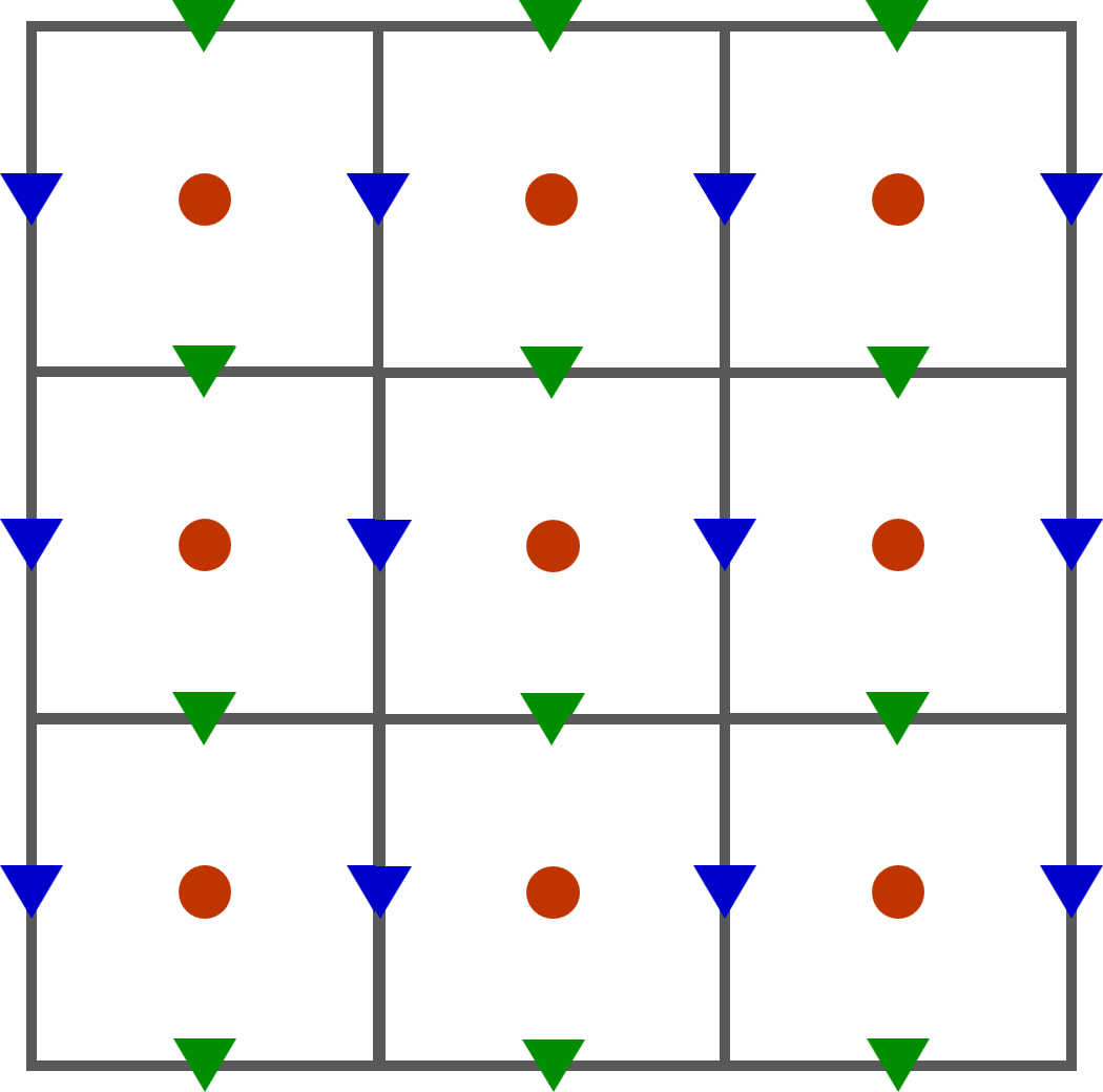
The cell_center grid convention assumes that field values ‘live’ at the center of each voxel (denoted by red dots in the figure below). Fluxes between two voxels are computed at so-called staggered field positions, i.e.

• x fluxes live on sides staggered to the right (blue)

• y fluxes live staggered to the top (green)

Initialize field with random noise

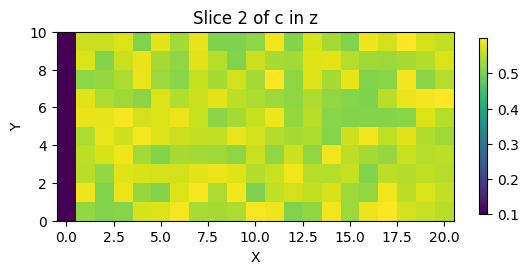
noise = 0.5 + 0.1*np.random.rand(Nx, Ny, Nz)
noise[0,:,:] = 0.1
vf.add_field("c", noise)

Explore plotting utilities of voxelFields class

%matplotlib inline
vf.plot_slice('c', 2, direction='z')

Interactive plotting to scroll through slices

# %matplotlib widget
# vf.plot_field_interactive("c", direction='x', colormap='turbo')

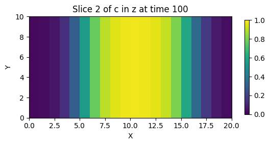
We can now plug the initial concentration field into the Periodic Cahn-Hilliard solver

%matplotlib inline
vf.add_field("c", noise)

end_time = 100
dt = 1
evo.run_cahn_hilliard_solver(
        vf, 'c', 'torch', jit='False', device='cuda',
        time_increment=dt, frames=10, max_iters=int(end_time/dt),
        verbose='plot', vtk_out=False, plot_bounds=(0,1))

Wall time: 8.4107 s after 100 iterations (0.0841 s/iter)
GPU-RAM (nvidia-smi)  current: 119 MB (119.0 MB max)
GPU-RAM (torch)       current: 8.13 MB (8.18 MB max, 22.00 MB reserved)

Export the final concentration field after solve to vtk

vf.export_to_vtk(filename='test.vtk')

Staggered grid positions

For some FFT solvers with mixed boundary conditions it is preferable to work with a staggered grid i.e. the node positions are shifted in a specific direction. To compute tortuosity, we utilize Dirichlet BCs in x-direction while the y- and z-direction are governed by zero-flux or periodic boundary conditions.

The VoxelFields object has the grid convention as an attribute which can be set to staggered_x. Note that there are now nodes located at the left and right boundary i.e. the grid spacing equals dx = Lx/(Nx-1) as exemplified below.

The field values are now stored at the blue positions.

Nx, Ny, Nz = [21, 10, 5]
vf = evo.VoxelFields((Nx, Ny, Nz), domain_size=(Nx-1, Ny, Nz), convention='staggered_x')
print("VoxelFields object is now defined as")
print(f" - grid with {vf.Nx} x {vf.Ny} x {vf.Nz} points,")
print(f" - defined with {vf.convention} grid convention.")
print(f" - Physical domain size {vf.domain_size}")
print(f" - and the resulting grid spacing {vf.spacing}")
print(f" - First grid point (origin) is located at {vf.origin}")
print(f" - Float precision of data is set to {vf.precision}")

VoxelFields object is now defined as
 - grid with 21 x 10 x 5 points,
 - defined with staggered_x grid convention.
 - Physical domain size (20, 10, 5)
 - and the resulting grid spacing (1.0, 1.0, 1.0)
 - First grid point (origin) is located at (0, 0.5, 0.5)
 - Float precision of data is set to float32

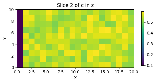
As this staggered grid positions are rather unusual, there is no 100% consistent way to visualize these fields. In a general sense, our data is still zonal data and will therefore be visualized with imshow in python and be exported using cell_data for the .vtk format. However, to highlight the difference, the origin is now shifted such that the first datapoints correlate with x=0 and the last with x=Lx.

noise = 0.5 + 0.1*np.random.rand(Nx, Ny, Nz)
noise[0,:,:] = 0.1
vf.add_field("c", noise)

%matplotlib inline
vf.plot_slice('c', 2, direction='z')