Differentiable numerical simulations

Both backends (torch and jax) naturally provide high computational performance based on just-in-time compiled kernels and end-to-end gradient-based parameter learning through automatic differentiation. This enables inverse material design where you start from a desired outcome (material behaviour or time evolution of a system) and work your way backwards to the input parameters which lead to this desired output. Generally, the integration of high-resolution imaging with predictive simulations and data‐driven optimization holds promise to accelerate discovery and to deepen our understanding of process–structure–property relationships.

Some general information about differentiable physics can be found here.

In the following example we build a physics-informed parameter estimation pipeline using differentiable simulation. The physical system is governed by the Cahn–Hilliard equation, a nonlinear fourth-order PDE modeling phase separation and coarsening in materials. It depends on two key parameters:

• \(D\) (mobility or diffusivity),

• \(\epsilon\) (controls interface thickness and energy).

We assume that the initial condition \(c_0(x)\) is known. A set of partial observations of the field \(c(x,t)\) at specific time steps \(t_i\) is given. The goal is to find the physical parameters (\(D\), \(\epsilon\)) that best reproduce the observed dynamics of \(c(x,t)\) across multiple sequences of the system’s evolution.

This is done by:

1. Simulating forward with guessed parameters to compute \(c_\text{sim}(x, t_i)\).

2. Computing residuals: difference between simulation and measurement.

3. Optimizing parameters: via Levenberg–Marquardt (a trust-region variant of Gauss–Newton least-squares).

Mathematically this can be expressed as

\[\min_\theta \sum_j^{N_\text{sequences}}\sum_i^{T} ||c_\text{measured}^{(j)}(t_i)−c_\text{sim}^{(j)}(t_i, \theta)||_2^2​\]

with the state variables \(\theta = (D, \epsilon)\).

import evoxels as evo
import numpy as np

Nx, Ny, Nz = [100, 100, 100]
vf = evo.VoxelFields((Nx, Ny, Nz), domain_size=(Nx, Ny, Nz))
noise = 0.5 + 0.1*(0.5-np.random.rand(Nx, Ny, Nz))
vf.add_field('c', noise)

We create an InversionModel for the CahnHilliard problem which sets up the voxel grid and the parameters of the PDE.

from evoxels.problem_definition import CahnHilliard
fixed_problem_kwargs={"mu_hom": None}
pos_params = ["D", "eps"]
model = evo.InversionModel(vf, CahnHilliard, pos_params, fixed_problem_kwargs)

Choose output times

diffrax.SaveAt specifies at which time points the solver should store the concentration field. These will later be used as training data.

import diffrax as dfx
saveat = dfx.SaveAt(ts=np.linspace(0, 100, 11))

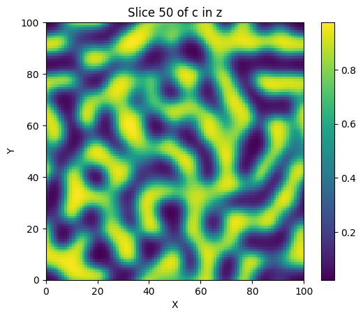
res = model.forward_solve({"D": 1.0, "eps": 3.0}, 'c', saveat, dt0=1)

Wall time: 3.2251 s after 100 iterations (0.0323 s/iter)
CPU-RAM (tracemalloc) current: 11.44 MB (15.20 MB max)
CPU-RAM (psutil)      current: 981.95 MB (0.00 MB max)
GPU-RAM (nvidia-smi)  current: 3791 MB (3791.0 MB max)

vf.plot_slice('c', Nz//2)

Next, the solver output is organised into a small dictionary containing the sampled states ys and their time stamps ts. The index list inds selects which time steps form each training sequence.

data = {}
data["ts"] = saveat.subs.ts
data["ys"] = res

inds = [[1,2,3], [4,5,6], [7,8,9]]

Run the optimisation

The train method performs a Levenberg–Marquardt least-squares fit of the parameters \(D\) and \(\epsilon\) so that the simulated states match the selected measurements.

tmp = model.train({"D": np.array([2.0]), "eps": np.array([2.0])}, data, inds, max_steps=50)

Step: 0, Accepted steps: 0, Steps since acceptance: 0, Loss on this step: 161784.984375, Loss on the last accepted step: 0.0, Step size: 1.0
Step: 1, Accepted steps: 1, Steps since acceptance: 0, Loss on this step: 30146.3125, Loss on the last accepted step: 161784.984375, Step size: 3.5
Step: 2, Accepted steps: 2, Steps since acceptance: 0, Loss on this step: 4532.947265625, Loss on the last accepted step: 30146.3125, Step size: 12.25
Step: 3, Accepted steps: 3, Steps since acceptance: 0, Loss on this step: 88.15148162841797, Loss on the last accepted step: 4532.947265625, Step size: 42.875
Step: 4, Accepted steps: 4, Steps since acceptance: 0, Loss on this step: 27.122346878051758, Loss on the last accepted step: 88.15148162841797, Step size: 42.875
Step: 5, Accepted steps: 5, Steps since acceptance: 0, Loss on this step: 27.092044830322266, Loss on the last accepted step: 27.122346878051758, Step size: 150.0625
Step: 6, Accepted steps: 6, Steps since acceptance: 0, Loss on this step: 27.092037200927734, Loss on the last accepted step: 27.092044830322266, Step size: 150.0625
Step: 7, Accepted steps: 7, Steps since acceptance: 0, Loss on this step: 27.0920352935791, Loss on the last accepted step: 27.092037200927734, Step size: 150.0625

The converged values from the physics-informed parameter estimation should be close to the ‘true’ values of \(D=1\) and \(\epsilon=3\). Even with the very small synthetic dataset used here the optimiser quickly converges.

print(f"Estimated D = {tmp['D']},")
print(f"Estimated eps = {tmp['eps']}.")

Estimated D = [0.92284304],
Estimated eps = [3.0126162].