Rapid prototyping for custom ODE classes
As a computational material scientist you might want to develop and test new PDEs for your specific application. Good general advice can be found in the recommended phase-field practices which - as the name says - is mainly focusing on phase-field methods but covers general aspects such as model formulation, numerical implementation, software development, etc.
Example: Reaction diffusion system (Gray-Scott model)
Note that this little example of a reaction diffusion system is based on the post by Karl Sims and the related work by Sebastian Lague. Thank you both for the inspiration!
Imagine two chemicals or species \(A\) and \(B\) which are dispersed in another medium. \(A\) is added at a given feed rate \(f\) but it can maximally reach a concentration of \(A=1\). A reaction converts one \(A\) into \(B\) in the presence of two other \(B\) (i.e. reaction term \(c_A c_B^2\)). \(B\) is continuously removed with a given kill rate \(k\) until it reaches \(B=0\). Both species are also diffusing within the solution with a given chemical diffusivity \(D_A\) and \(D_B\) respectively.
The coupled behaviour of both species can be formulated in terms of the coupled PDEs:
A variation of the input parameters (feed rate, kill rate and the ratio of diffusivities) leads to a wide range of different results. Let’s explore how surprisingly complex and dynamic the emerging behaviours can be given such simple rules…
Defining the custom ODE class
evoxels comes with predefined ODE classes for phase evolution and reaction-diffusion system but we can also use the modular concept to prototype new systems of PDEs. This generally involves:
Formulation of the analytical right-hand side in sympy logic
Discretisation of the rhs into an ODE system using finite differences
Defining the expected order of convergence
Testing if the implementation is correct and achieves the expected order of convergence before simulating the material behaviour.
For our chosen exmple - the Gray-Scott model:
We define the for parameters \(D_A\), \(D_B\), \(f\) and \(k\) as input paramters. Additionally, the interaction term is set to \(c_A c_B^2\) by default but can also be given as an input function.
The
CoupledReactionDiffusionclass inherits from theSemiLinearODEclass because we want to use thePseudoSpectralIMEXtimestepper later on. Therefore, we need to define the spectral factor which is defined as the factor in front of the laplacian term multiplied by the squared wave vectorsk.The
interactionterm takeslibas an additional input argument to make it compatible with both the analytical and numerical evaluation of the right-hand side. In the first case we inputsympyas the library and, in the second case, the backend library (torch/jax) is used.
[1]:
from dataclasses import dataclass, field
from typing import Any, Callable
import sympy as sp
import sympy.vector as spv
from evoxels.problem_definition import SemiLinearODE
from evoxels.voxelgrid import VoxelGrid

@dataclass
class CoupledReactionDiffusion(SemiLinearODE):
    vg: VoxelGrid
    D_A: float = 1.0
    D_B: float = 0.5
    feed: float = 0.055
    kill: float = 0.117
    interaction: Callable | None = None
    _fourier_symbol: Any = field(init=False, repr=False)

    def __post_init__(self):
        """Precompute factors required by the spectral solver."""
        self.initialize_boundary_conditions()
        self._fourier_symbol = - max(self.D_A, self.D_B) * self.k_squared()
        if self.interaction is None:
            self.interaction = lambda u, lib=None: u[0] * u[1]**2

    @property
    def order(self):
        return 2

    @property
    def fourier_symbol(self):
        return self._fourier_symbol

    def _eval_interaction(self, u, lib):
        """Evaluate interaction term"""
        try:
            return self.interaction(u, lib)
        except TypeError:
            return self.interaction(u)

    def rhs_analytic(self, t, u):
        interaction = self._eval_interaction(u, sp)
        dc_A = self.D_A*spv.laplacian(u[0]) - interaction + self.feed * (1-u[0])
        dc_B = self.D_B*spv.laplacian(u[1]) + interaction - self.kill * u[1]
        return (dc_A, dc_B)

    def rhs(self, t, u):
        r"""Two-component reaction-diffusion system

        Use batch channels for multiple species:
        - Species A with concentration c_A = u[0]
        - Species B with concentration c_B = u[1]

        Args:
            u (array-like): species
            t (float): Current time.

        Returns:
            Backend array of the same shape as ``u`` containing ``du/dt``.
        """
        interaction = self._eval_interaction(u, self.vg.lib)
        u_pad = self.pad_bc(u)
        laplace = self.vg.laplace(u_pad)
        dc_A = self.D_A*laplace[0] - interaction + self.feed * (1-u[0])
        dc_B = self.D_B*laplace[1] + interaction - self.kill * u[1]
        return self.vg.lib.stack((dc_A, dc_B), 0)
Testing the right-hand side
Before running simulations, we should test whether the implementation of our equations is correct and achieves the expected order of convergence or not. Let’s define the test functions, i.e. two initial fields for \(c_A\) and \(c_B\) which must comply with the boundary conditions of our ODE, i.e. periodicity in this case.
[2]:
import sympy as sp
import sympy.vector as spv

CS = spv.CoordSys3D('CS')
test_funs = (0.5 + 0.3 * sp.cos(4*sp.pi*CS.x) * sp.cos(4*sp.pi*CS.y)**3,
             0.4 + 0.1 * sp.sin(2*sp.pi*CS.x) * sp.cos(4*sp.pi*CS.z) )
The convergence test for ODE right-hand sides is predefined in the utils.py file and can be imported - fully ready to be used:
[3]:
from evoxels.utils import rhs_convergence_test

precision = 'float64'
dx, errors, slope, order = rhs_convergence_test(
        ODE_class      = CoupledReactionDiffusion,
        problem_kwargs = {"D_A": 1.0, "D_B": 0.5},
        test_function  = test_funs,
        convention     = 'cell_center',
        dtype          = precision
    )

print(f"Grid spacing: {dx}")
print(f"Errors c_a:   {errors[0]}")
print(f"Errors c_b:   {errors[1]}")
print("Convergence rate from slope fit:", slope)
print("Expected order of convergence:  ", order)
Grid spacing: [0.125     0.0625    0.03125   0.015625  0.0078125]
Errors c_a:   [1.81181187 0.30247238 0.08655272 0.02238807 0.00564499]
Errors c_b:   [0.16207643 0.04296587 0.01090076 0.00273525 0.00068444]
Convergence rate from slope fit: [2.04084953 1.97485054]
Expected order of convergence:   2
Let’s now visualise the resulting order of convergence as an error plot over the spatial discretisation \(\Delta x\) with logarithmic axes.
[4]:
import matplotlib.pyplot as plt

plt.loglog(dx, errors[0],'*')
plt.loglog(dx, errors[1],'+')
plt.loglog(dx, errors[0,0]/dx[0]**0.5*dx**0.5, '--', label = 'order 0.5')
plt.loglog(dx, errors[0,0]/dx[0]*dx,'--', label = 'order 1')
plt.loglog(dx, errors[0,0]/dx[0]**1.5*dx**1.5,'--', label = 'order 1.5')
plt.loglog(dx, errors[0,0]/dx[0]**2*dx**2,'--', label = 'order 2')
plt.loglog(dx, errors[1,0]/dx[0]**2*dx**2,'--', label = 'order 2')
plt.legend()
plt.title(f'Test for full_rhs with precision {precision}')
plt.show()
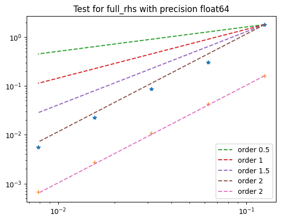
Hurray! Our CoupledReactionDiffusion is correctly implemented and shows second order convergence as expected.
Run simulations
Now that the new ODE class is fully implemented and tested, let’s have some fun with simulations. In order to run simulations we
Instantiate a VoxelFileds class
Create two initial fields for \(c_A\) and \(c_B\)
Set the problem-specific input parameters
Create a solver based on a given backend (
torch), our ODE class and a predefined timestepper (PseudoSpectralIMEX)`Run the solve function for a defined amount of timesteps with given \(\Delta t\) and the amount of frames. Set
verbose='plot'for on-the-fly visualisation and choose a custom colorbar (e.g.'turbo').
Have fun!
[5]:
import evoxels as evo
import numpy as np
import torch
from evoxels.solvers import TimeDependentSolver
from evoxels.timesteppers import PseudoSpectralIMEX

Nx, Ny, Nz = [700, 700, 1]
vf = evo.VoxelFields((Nx, Ny, Nz), domain_size=(Nx, Ny, Nz))
vf.add_field('c_a', np.ones((Nx, Ny, Nz)))
vf.add_field('c_b')

vf.set_voxel_sphere('c_b', (Nx//4, Ny//4, Nz//2), 5, 1)
vf.set_voxel_sphere('c_b', (Nx//4, Ny//4-3, Nz//2), 5, 0)

# stripes and bubbles: D_b=0.2, feed=0.053, kill=0.1165
# rings and bubbles: D_b=0.2, feed=0.055, kill=0.11
# cells D_b=0.2, feed=0.055, kill=0.14
# corals D_b=0.5, feed=0.055, kill=0.117
# waves D_b=0.5, feed=0.012, kill=0.06
problem_kwargs = {\
    "D_A": 1.0, "D_B": 0.2,
    "feed": 0.055,
    "kill": 0.11
}
solver = TimeDependentSolver(
        vf, ('c_a', 'c_b'),
        'torch', device='cuda',
        problem_cls = CoupledReactionDiffusion,
        timestepper_cls = PseudoSpectralIMEX,
    )
solver.solve(1, 50, 10000, problem_kwargs, verbose='plot', colormap='turbo')
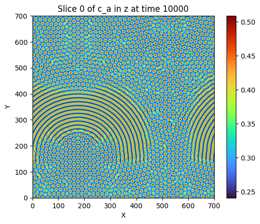
Wall time: 38.3455 s after 10000 iterations (0.0038 s/iter)
GPU-RAM (nvidia-smi)  current: 434 MB (434.0 MB max)
GPU-RAM (torch)       current: 16.26 MB (47.74 MB max, 66.00 MB reserved)
As a little cherry on the cake, we can modify the interaction term between the two species to make the reaction \(A\to B\) faster/slower in particular areas. For this we create a meshgrid (carefull: this must be on the same device as the VoxelGrid in the solver) and modify the original interaction term \(c_A c_B^2\) to
[6]:
vf.add_field('c_a', np.ones((Nx, Ny, Nz)))
vf.add_field('c_b')

vf.set_voxel_sphere('c_b', (Nx//4, Ny//4, Nz//2), 5, 1)
# vf.set_voxel_sphere('c_b', (Nx//4, Ny//4-3, Nz//2), 5, 0)

axes = tuple(torch.arange(0, n, device='cuda') * vf.spacing[i] + vf.origin[i]
                     for i, n in enumerate(vf.shape))
grid = tuple(torch.meshgrid(*axes, indexing='ij'))

def interaction(u, lib):
    return u[0] * u[1]**2 * (1 - 0.2*lib.cos(4*lib.pi*grid[0]/Nx)*lib.cos(2*lib.pi*grid[1]/Ny))

problem_kwargs = {\
    "D_A": 1.0, "D_B": 0.2,
    "feed": 0.055,
    "kill": 0.11,
    "interaction": interaction}

solver = TimeDependentSolver(
        vf, ('c_a', 'c_b'),
        'torch', device='cuda',
        problem_cls = CoupledReactionDiffusion,
        timestepper_cls = PseudoSpectralIMEX,
    )
solver.solve(1, 50, 10000, problem_kwargs, verbose='plot', colormap='turbo')
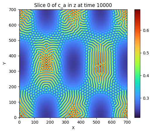
Wall time: 37.7972 s after 10000 iterations (0.0038 s/iter)
GPU-RAM (nvidia-smi)  current: 434 MB (434.0 MB max)
GPU-RAM (torch)       current: 16.27 MB (47.75 MB max, 66.00 MB reserved)
Eager to try out more? Here are some ressources of inspiring work: